
Volume 13, Issue 1 (3-2025)
Jorjani Biomed J 2025, 13(1): 3-14 |
Back to browse issues page


![]()
![]()
![]()
Download citation:
BibTeX | RIS | EndNote | Medlars | ProCite | Reference Manager | RefWorks
Send citation to:


BibTeX | RIS | EndNote | Medlars | ProCite | Reference Manager | RefWorks
Send citation to:
Shariaty H, Bagheri F. Enhanced missing value imputation and gaussian mixture model-based semi-supervised learning for predicting type 2 diabetes. Jorjani Biomed J 2025; 13 (1) :3-14
URL: http://goums.ac.ir/jorjanijournal/article-1-1050-en.html
URL: http://goums.ac.ir/jorjanijournal/article-1-1050-en.html


1- Department of Computer Engineering, Faculty of Engineering, Golestan University, Gorgan, Iran
2- Department of Computer Engineering, Faculty of Engineering, Golestan University, Gorgan, Iran ,f.bagheri@gu.ac.ir
2- Department of Computer Engineering, Faculty of Engineering, Golestan University, Gorgan, Iran ,
Keywords: Diabetes Mellitus, Machine Learning, Prediction Algorithms, Gaussian Mixture Model, Random Forest
Full-Text [PDF 1295 kb]
(2563 Downloads)
| Abstract (HTML) (9801 Views)
Methods
Previous studies have emphasized the importance of addressing missing data as a critical step in classification methods due to the frequent occurrence of missing values in the PIMA dataset. This research paper proposes a novel semi-supervised approach for predicting diabetes. Initially, a data imputation model utilizing clustering techniques is introduced to improve the handling of missing values. An integration of clustering and classification methods is then proposed to predict diabetes status. The application of this semi-supervised preprocessing and classification approach has culminated in enhanced prediction performance.
Our method consists of two main stages: data preprocessing and classification. The dataset contains numerous missing values; therefore, proposing an effective approach to address this issue can significantly enhance the subsequent stages. Furthermore, the classification approach that is both effective and well-designed for the specific data warrants careful consideration.
Figure 1 illustrates the schematic of the proposed semi-supervised approach. The subsequent sections of this part of the paper will provide in-depth explanations and analyses of each stage, facilitating a comprehensive understanding of the proposed methodology.
The following section outlines the utilized techniques and machine learning algorithms employed, followed by a comprehensive introduction of the proposed method.
Utilized techniques and machine learning models
The research paper employs various machine learning models to predict diabetes. The models utilized in this study include the Gaussian mixture model (GMM) and RF. Each model is briefly introduced below.
Gaussian Mixture Model: GMM clustering is a probabilistic model that assumes data is generated from a mixture of Gaussian distributions. It is widely utilized for clustering and density estimation tasks. A Gaussian Mixture Model is an unsupervised clustering method that identifies clusters by estimating probability densities through the Expectation-Maximization process, resulting in ellipsoidal shapes. In the Gaussian Mixture Model, each cluster is defined as a Gaussian distribution characterized by both the mean and covariance, in contrast to K-Means, which considers only the mean. GMMs possess this characteristic, enabling them to provide a more accurate quantitative assessment of fitness based on the number of clusters. While K-Means is well-known for its simplicity and computational efficiency, it may not fully capture the inherent diversity of the data. Gaussian Mixture Models excel at identifying complex patterns and organizing them into coherent, uniform elements that accurately reflect the underlying patterns present in the dataset (27).
Random Forest: The RF algorithm is a supervised learning technique that constructs an ensemble of DT. Each DT in the ensemble is trained on a random subset of the data, and the final prediction is determined through majority voting or averaging. RF can effectively handle high-dimensional data and is resistant to overfitting. It leverages the collective decisions of multiple DTs to deliver accurate and reliable predictions in both classification and regression scenarios. The ensemble approach, combined with random feature sampling, is essential for creating diverse and efficient models (28).
The proposed semi-supervised approach for diabetes prediction
The proposed semi-supervised approach for forcasting diabetes consists of two main stages: Data preprocessing and classification. Given the frequent occurrence of missing data in the PIMA dataset, the implementation of a clustering-based data imputation model is essential for resolving this challenge. This initial step improves the quality of the dataset by imputing missing values using a robust clustering mechanism, thereby preparing the data for next classification tasks.
Following the data preprocessing stage, an innovative integration of clustering and classification techniques is proposed to predict diabetes status. By leveraging the strengths of both clustering and classification, this approach aims to improve the accuracy and reliability of diabetes prediction. The application of this semi-supervised preprocessing and classification approach has yielded promising results in terms of predictive performance, as demonstrated in the experimental evaluation.
The PIMA dataset was utilized to test the proposed approach. It includes various features such as glucose levels, blood pressure, skin thickness, insulin levels, body mass index (BMI), age, and diabetes status for 768 women, some of which contain missing values. A clustering-based method is recommended for imputing these missing values, considering their critical importance in the dataset. The dataset comprises both diabetic and non-diabetic classes, and the primary challenge lies in accurately predicting these classifications.
To ensure consistent scaling of the variables, normalization has been applied to the values. However, because zero values (As missing data) disrupt the normalization of features that should not include zero values, this process has been carried out without accounting for those zeros. Equation 1 is used to normalize the features.

WhereX max X min X X '
Results
Datasets
The PIMA Indian dataset utilized in this research comprises information from 768 instances of adult women aged 21 and older. This dataset includes various features, such as glucose level, blood pressure, skin thickness, insulin level, BMI, age, and diabetes status named" outcome" which indicates whether an individual has diabetes (1) or does not have diabetes (1 or 0).
Based on the available data, it can be observed that 65.1% of the patients in the dataset are categorized as non-diabetic, while 34.9% are identified as diabetic. Table 2 provides a description of the PIMA Indian dataset. A heat map illustrating the Pearson correlation coefficients for all diabetes-related characteristics is presented in Figure 4, demonstrating the relationships between the various variables in the dataset.
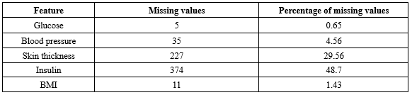
It is important to acknowledge that certain attributes, like" Pregnancy", may contain zero values, while others must not include zero values to maintain data validity. The frequency of zero values in the features is presented in Table 3. Based on the information in Table 3, it is evident that both insulin and glucose have a substantial number of missing values. Given the nature of the dataset and the specific characteristics of diabetes, it is essential to address these zero values appropriately during data preprocessing.
Evaluation
The performance of the classification algorithm was evaluated using various metrics, such as accuracy, precision, recall and F1-score. These metrics will be briefly explained in the following sections.
Accuracy: This is calculated by dividing the total number of correct predictions by the total number of predictions. It can be expressed as follows:

Precision (Positive Predictive Value (PPV)): This term refers to the proportion of true positive (TP) diagnoses of diabetic patients out of all samples that the model classified as diabetic, regardless of whether these classifications were correct (TP) or incorrect (False positives (FP)).

Recall (Sensitivity Rate): This term is defined as the proportion of correctly diagnosed diabetic patients (TP) out of all actual diabetic cases in the dataset, including both those correctly identified by the model (TP) and those that were missed (False negatives (FN)).

F1-Score: The F1-score is a metric that combines precision and recall, taking into account both false positives (FP) and FN.

Missing value imputation
In this paper, we introduced a new unsupervised imputation method based on clustering. The first step involved separating records without missing values (Reference data) from the datasets. These reference records were employed to impute missing values in the remaining records.
Initially, all reference data were clustered using the GMM algorithm. The clustering analysis was conducted with various numbers of clusters (k), and the results are presented in Table 4. One important measure for evaluating cluster quality is ensuring adequate separation, which minimizes variability between diabetic and non-diabetic patients within each cluster.
Upon examining different clusters, it was observed that a significant proportion of individuals without diabetes were grouped together in one cluster, while those with diabetes were distributed among different groups alongside non-diabetic individuals. Consequently, two clusters (k=2) were deemed most suitable for the proposed MVI method. Subsequently, these two scenarios were utilized to fill in the missing values in the dataset.
To evaluate the impact of the proposed method for imputing missing values on the accuracy of classification results, various classification techniques have been employed alongside different strategies for handling missing data.
A comparison was conducted using various algorithms, including SVM, RF, DT and our classification approach. Additionally, different data imputation techniques were employed, such as removing records with missing values, filling in missing values with the average, and utilizing the proposed method for imputing missing values. The results of this comparison are presented in Table 5.
The experimental findings revealed that the proposed MVI method for significantly improved the accuracy of these classification techniques.
The proposed classification method
The PIMA dataset comprises two groups: "Diabetics," referring to individuals diagnosed with diabetes, and "non-diabetics," referring to those without diabetes. The dataset exhibits an imbalanced class distribution, with approximately 65.1% of the records categorized as "non-diabetics" and 34.9% categorized as "diabetics."
To achieve an even distribution of classes in both the train and test sets, a balanced sampling method is employed. For this purpose, a random selection of 70% of the "non-diabetics" class records and 70% from the "diabetics" class is used to create the train dataset. This ensures that our training dataset preserves the original class distribution of the data. The remaining 30% of records, which include both "diabetic" and "non-diabetic" entries form the test set.
This stratified random sampling enables us to maintain the original class distribution in both the train and test sets, thereby facilitating effective training and evaluation of classification methods for both classes. The testing dataset offers an unbiased assessment of the classification model’s performance, considering class imbalances that are similar to those in the train set.
The model was implemented using Python 3.11 within the PyCharm 2022.3.3 development environment. A variety of Python libraries were employed to facilitate different aspects of the workflow, including openpyxl, Numpy, scikit-learn, Matplotlib, pandas, seaborn, and Python's built-in random module for stratified sampling. Each machine learning model was evaluated under various hyperparameter configurations. The random forest algorithm, with a maximum depth of 5 and 50 estimators, achieved the best performance during hyperparameter tuning. Furthermore, both cross-validation and stratified random sampling were employed, with each method being conducted five.
The adjustments to the proposed classification method are detailed below.
Clustering the train dataset: The train dataset is clustered using the GMM method with different numbers of clusters (k), ranging from 2 to 5. This analysis reveals that how the records are distributed among the clusters. Moreover, this examination shows the distribution of records across the clusters, and each clustering implementation with k clusters yields different distributions of " diabetic" and" non-diabetic" records within the clusters. This clustering analysis helps us understand the underlying patterns within the train dataset and how the" diabetics" and" non-diabetics" records are distributed among the clusters. The outcomes of clustering implementation with different numbers of clusters are presented in Table 6.
Choosing the optimal clusters: According to the clustering results, the train datasets are divided into three clusters (k=3), as illustrated in Table 6. The second cluster (C_2) contains more "non-diabetic" records and the third one (C_3) contains a greater number of "diabetic" records. These two clusters are utilized for classification purposes. The first cluster (C_1) consists of a mixture of "diabetic" and "non-diabetic" records. This heterogeneous cluster is excluded from this stage of the classification process, as it does not provide clear guidance for classifying the test records. A two-dimensional (2D) plot of the clusters is presented is Figure 5 based on Glucose and BMI for better visualization. These two variables were chosen due to their significant impact on the outcome, as indicated by the heatmap in Figure 4.
The total number of records in the two clusters-diabetics and non-diabetics-used as the basis for classification is 366.
Classification of test data based on two specified clusters: To classify the test data, the distances between each test data point and all data points within the "diabetic" and "non-diabetic" clusters are calculated. The label for the test data is assigned based on the nearest data point within these two clusters.
To further validate these assignments based on distances, a threshold is taken into account. If the test data point is closer to the "diabetic" cluster and the distance from the test data to this cluster is less than a specific threshold, labeled as "diabetics". Similarly, if it is nearer to the "non-diabetic" cluster and also meets the distance threshold, it is classified as "non-diabetic."
The experiments were conducted across a range of threshold values from 0.1 to 1, and the classification performance was assessed and presented in Table 7.
Choosing the optimal threshold: It is important to identify an optimal threshold that minimizes the rate of rejected data while maintaining high accuracy. Striking a balance between these factors is essential; therefore, we have selected a threshold value of 0.4 in order to achieve a lower rejection rate with minimal impact on accuracy.
Rejection rate of unclassifiable data: Test data points whose distance to the nearest "diabetic" or "non-diabetic" category exceeds the specified threshold are labeled as "rejected". The classifications of these instances become uncertain due to their proximity to the selected cluster data points.
The rejection rate of the algorithm is calculated as the proportion of data that could not be classified in the previous stage. These rates for different threshold values are computed and presented in Table 7.
Rejected data points classification: The evaluation of the algorithm can be conducted solely on labeled data without considering the rejected data points. To improve the efficiency of the proposed algorithm, a separate mechanism is also implemented to classify the rejected data.
According to the experimental results presented in Table 5, the random forest algorithm demonstrated superior classification performance compared to other machine learning algorithms. Consequently, this particular algorithm was selected for classifying rejected data points.
Full-Text: (1074 Views)
Introduction
Diabetes is a prevalent condition that currently has no permanent cure and is often referred to as a "silent killer." Effectively managing prediabetes can prevent its progression to full-blown diabetes. A lack of understanding about this condition can lead to additional complications and challenges (1).
Diabetes is generally classified into three categories: Type I, Type II, and gestational diabetes. In Type I diabetes, the immune system attacks and damages the insulin-producing cells. In contrast, Type II diabetes, which is more common than Type I, arises when the body fails to respond effectively to the insulin that is produced, leading to elevated blood sugar levels (2,3).
Diabetes symptoms can manifest suddenly, often characterized by increased thirst, frequent urination, blurred vision, fatigue, and unexplained weight loss. Over time, diabetes can damage various organs, including the heart, eyes, kidneys, nerves, and blood vessels, thereby increasing the risk of severe health complications, such as heart attacks, strokes, and kidney failure. Additionally, diabetes is associated with complications like vision impairment and foot ulcers, which may lead to amputation, earning it the moniker "silent killer" (2-5).
In 2014, approximately 8.5% of the global adult population was affected by diabetes, which poses a significant public health concern. By 2019, this condition was directly responsible for 1.5 million deaths, particularly among individuals under the age of 70. The mortality rate attributed to diabetes increased by 3% between 2000 and 2019, with a notable rise of 13% in lower-middle-income countries. On a positive note, there was a global decrease of 22% in the likelihood of premature death caused by diabetes and other noncommunicable diseases from 2000 to 2019 (5).
Recent studies demonstrate that approximately 80% of complications related to Type 2 diabetes can be prevented or delayed through early identification and intervention for at-risk individuals. Advanced data analysis methods, such as data mining and machine learning, offer promising opportunities for identifying those at risk. Various techniques in data mining and machine learning have been developed and implemented to improve the diagnosis and management of diabetes (6-12).
Various approaches, including decision trees (DTs), neural networks (NN), support vector machines (SVMs), and ensemble methods, have emerged in the fields of data mining and machine learning. These methodologies are employed to analyze a diverse array of data, such as medical records, genetic information, lifestyle factors, and clinical markers. Their objective is to detect patterns and variables related to diabetes and its associated adverse effects. By utilizing advanced data analysis techniques, we have made remarkable progress in the early detection and management of individuals at risk for diabetes. These approaches substantially contribute to interpreting widespread datasets, uncovering processes and potential risk factors, and proposing feasible interventions. Finally, they contribute to improving diabetes care and reducing associated adverse effects (6-12).
In this study, we present a new machine-learning model designed to improve the accuracy of diabetes prediction through a novel approach for handling missing values and a classification method. The paper begins with an overview of previous research studies on the PIMA dataset in Section 2, which discusses various methodologies employed by other researchers. Section 3 presents a comprehensive analysis, starting with clustering and outlining our proposed methodology. Section 4 introduces the dataset, investigates missing value imputation (MVI), and assesses alternative classification techniques. In Section 5, we analyze how the MVI approach and the proposed classifier elevate performance.
In this section, we review the existing literature related to the subject in order to analyze and differentiate their methodologies from the approach presented in this study. Previous research has proposed a variety of methods.
Rajni and Amandeep employed the recursive Bayesian (RB) algorithm in their research to predict the risk of diabetes, utilizing the PIDD as their primary data source. Their proposed method achieved an accuracy rate of 72.9% (13).
Lella et al. proposed a predictive model classified as an A-type unorganized Turing machine (UTM), which functions through a system of combinational NAND gates. Their model achieved an accuracy rate of 80.1% on the PIMA Indians Diabetes Database (PIDD) (14).
Benarbia conducted a study utilizing four distinct machine learning algorithms: Logistic regression (LR), DT, random forest (RF), and SVM for data modeling. The research involved implementing these algorithms on both scaled and unscaled datasets. Among all the algorithms employed, the highest accuracy of 82% was achieved by the LR algorithm on the PIMA dataset (15).
Huang and Ruodi utilized machine learning techniques on the PIDD to predict diabetes in individuals. Their study concluded that the extreme gradient boosting algorithm was the most effective model, exhibiting an accuracy rate of 82.29% (16).
Chang et al. analyzed the PIDD using three machine learning algorithms: the J48 DT, RF, and naïve Bayes (NB). Their research revealed that the RF algorithm exhibited the highest performance, achieving an accuracy rate of 79.57% (17).
Alam et al. employed a variety of algorithmic techniques, including artificial neural networks (ANN), RF, and k-means clustering for their analysis. Among these methodologies, the ANN yielded the most favorable results, achieving an accuracy of 75.7% (18).
Singh and Singh utilized the NSGA-II-Stacking approach, an advanced method that demonstrates superiority over individual machine-learning techniques and traditional ensemble tactics. Their proposed system excels in performance assessment, achieving an accuracy of 83.8% (19).
Maniruzzaman et al. employed several classification techniques, including linear discriminant analysis (LDA), quadratic discriminant analysis (QDA), and NB. They also adapted Gaussian process-based classification techniques to enhance the accuracy of diabetes diagnosis, achieving an accuracy rate of 81.97% (20).
Kumari et al. conducted an investigation utilizing various machine learning models, including RF, LR, and NB. These models were integrated into a soft voting classifier to effectively classify and predict diabetes. To enhance data quality, the researchers applied essential preprocessing methods, such as replacing missing attribute values with their medians. The accuracy of their proposed method was 79.04% when evaluated on the PIMA dataset (21).
Rajendra and Latif employed various methods, including LR and Max Voting, to evaluate accuracy across diverse scenarios using two datasets, one of which was the PIMA Indian dataset. The highest level of accuracy achieved with the PIMA dataset was 78%, utilizing the Max Voting method (22).
Saxena et al. employed feature selection and data preprocessing techniques to improve the classification process. They implemented several classification algorithms, including K-nearest neighbors (KNN), RF, DTs, and multilayer perceptron (MLP). Their approach culminated in an accuracy of 79.8% when tested on the PIMA dataset using RF (23).
Tiggaa and Shruti employed various classification methods, including LR, KNN, SVM, NB, DT, and RF. Among these classifiers, the Random Forest algorithm demonstrated the most robust performance, achieving an accuracy rate of 75% when applied to the PIMA dataset (24).
Chang et al. conducted an analysis of the PIDD using three distinct machine learning models: J48 DT, RF, and NB. The Random Forest model exhibited the highest performance, achieving an accuracy rate of 79.57% (25).
Jackins et al. employed the NB and RF classification algorithms to predict clinical diseases. The highest level of accuracy, 74.46%, was achieved using the RF algorithm on the PIMA dataset (26).
Prior studies have highlighted the importance of addressing missing data as a critical step in classification methods due to the frequent occurrence of missing values in the PIMA dataset. The reviews summarized in Table 1 focus on the use of feature selection and MVI methods when working with the PIMA dataset.
|
Table 1. Summary of related works on PIMA dataset
 FS: Feature Selection; MVI: Missing Value Imputation; KNN: K-Nearest Neighbors; PCA: Principal Component Analysis; SVM: Support Vector Machine; DT: Decision Tree; NB: Naïve Bayes; RB-Bayes: Recursive Bayesian; LR: Logistic Regression; RF: Random Forest; ANN: Artificial Neural Networks; NSGA: Non-dominated Sorting Genetic Algorithm; LDA: Linear Discriminant Analysis; QDA: Quadratic Discriminant Analysis; GPC: Granite Powder Concrete; MLP: Multilayer Perceptron; EBBM-based UTM: Evolutionary Bait Balls Model-based Unorganized Turing Machine; KNN: K-Nearest Neighbor |
Methods
Previous studies have emphasized the importance of addressing missing data as a critical step in classification methods due to the frequent occurrence of missing values in the PIMA dataset. This research paper proposes a novel semi-supervised approach for predicting diabetes. Initially, a data imputation model utilizing clustering techniques is introduced to improve the handling of missing values. An integration of clustering and classification methods is then proposed to predict diabetes status. The application of this semi-supervised preprocessing and classification approach has culminated in enhanced prediction performance.
Our method consists of two main stages: data preprocessing and classification. The dataset contains numerous missing values; therefore, proposing an effective approach to address this issue can significantly enhance the subsequent stages. Furthermore, the classification approach that is both effective and well-designed for the specific data warrants careful consideration.
Figure 1 illustrates the schematic of the proposed semi-supervised approach. The subsequent sections of this part of the paper will provide in-depth explanations and analyses of each stage, facilitating a comprehensive understanding of the proposed methodology.
The following section outlines the utilized techniques and machine learning algorithms employed, followed by a comprehensive introduction of the proposed method.
Utilized techniques and machine learning models
The research paper employs various machine learning models to predict diabetes. The models utilized in this study include the Gaussian mixture model (GMM) and RF. Each model is briefly introduced below.
Gaussian Mixture Model: GMM clustering is a probabilistic model that assumes data is generated from a mixture of Gaussian distributions. It is widely utilized for clustering and density estimation tasks. A Gaussian Mixture Model is an unsupervised clustering method that identifies clusters by estimating probability densities through the Expectation-Maximization process, resulting in ellipsoidal shapes. In the Gaussian Mixture Model, each cluster is defined as a Gaussian distribution characterized by both the mean and covariance, in contrast to K-Means, which considers only the mean. GMMs possess this characteristic, enabling them to provide a more accurate quantitative assessment of fitness based on the number of clusters. While K-Means is well-known for its simplicity and computational efficiency, it may not fully capture the inherent diversity of the data. Gaussian Mixture Models excel at identifying complex patterns and organizing them into coherent, uniform elements that accurately reflect the underlying patterns present in the dataset (27).
Random Forest: The RF algorithm is a supervised learning technique that constructs an ensemble of DT. Each DT in the ensemble is trained on a random subset of the data, and the final prediction is determined through majority voting or averaging. RF can effectively handle high-dimensional data and is resistant to overfitting. It leverages the collective decisions of multiple DTs to deliver accurate and reliable predictions in both classification and regression scenarios. The ensemble approach, combined with random feature sampling, is essential for creating diverse and efficient models (28).
The proposed semi-supervised approach for diabetes prediction
The proposed semi-supervised approach for forcasting diabetes consists of two main stages: Data preprocessing and classification. Given the frequent occurrence of missing data in the PIMA dataset, the implementation of a clustering-based data imputation model is essential for resolving this challenge. This initial step improves the quality of the dataset by imputing missing values using a robust clustering mechanism, thereby preparing the data for next classification tasks.
Following the data preprocessing stage, an innovative integration of clustering and classification techniques is proposed to predict diabetes status. By leveraging the strengths of both clustering and classification, this approach aims to improve the accuracy and reliability of diabetes prediction. The application of this semi-supervised preprocessing and classification approach has yielded promising results in terms of predictive performance, as demonstrated in the experimental evaluation.
The PIMA dataset was utilized to test the proposed approach. It includes various features such as glucose levels, blood pressure, skin thickness, insulin levels, body mass index (BMI), age, and diabetes status for 768 women, some of which contain missing values. A clustering-based method is recommended for imputing these missing values, considering their critical importance in the dataset. The dataset comprises both diabetic and non-diabetic classes, and the primary challenge lies in accurately predicting these classifications.
To ensure consistent scaling of the variables, normalization has been applied to the values. However, because zero values (As missing data) disrupt the normalization of features that should not include zero values, this process has been carried out without accounting for those zeros. Equation 1 is used to normalize the features.
Where
The Proposed Clustering-Based Unsupervised Approach for Missing Value Imputation
There are several methods available to address missing values in datasets. One commonly used strategy for handling missing values in a dataset is to remove all records that contain missing values in at least one feature. However, this approach can culminate in the loss of important records and valuable information, particularly when applied to the PIMA dataset.
Another commonly used approach to address missing values is to impute them using the mean or median. However, it is important to note that these methods can potentially introduce bias into the data (29).
Addressing missing values is an essential step in the preprocessing of data, particularly when working with datasets that contain a substantial number of missing entries.
In this paper, we propose a novel clustering-based unsupervised approach for imputing missing values. The first step involves segregating the records without any missing values, referred to as reference data, from the datasets. These records will serve as references for imputing missing values in the remaining records that contain one or more missing values.
In the first phase, all reference data are clustered using GMM algorithm. One of the advantages of utilizing this algorithm is its capability to effectively distinguish between clusters with non-spherical shapes.
 Figure 1. The proposed framework for diabetes prediction |
The clustering analysis was conducted using various numbers of clusters (k) and the findings are detailed in the results section. A key measure for evaluating the quality of clustering is ensuring that samples are sufficiently separated, resulting in low variability between diabetic and non-diabetic patients within each cluster. Essentially, it should be possible to form clusters in which a majority of individuals belong to either the diabetic or non-diabetic category.
By examining various clusters, it was observed that a significant proportion of individuals without diabetes were grouped together in one cluster. In contrast, individuals with diabetes were not distinctly categorized into a separate cluster; instead, they were distributed among different groups alongside non-diabetic individuals. Therefore, the clusters resulting from the analysis using two clusters (k=2) are the most appropriate choice for the proposed MVI method. The details of Cluster 1 and Cluster 2, derived from the clustering with k=2, are presented below.
Cluster 1 consists of 87% non-diabetic individuals and 13% diabetic individuals (C 1  with the majority of samples being non-diabetic (
x nd  ) and a smaller number of samples being diabetic (
x d  ),
), x 1  (i) ∈
(i) ∈ C 1
Cluster 2 consists of 45% non-diabetic and 55% diabetic individuals (C 2  represented by a mixture of
 x nd x d x 2  (i) ∈
(i) ∈ C 2
Cluster 1 primarily consists of individuals without diabetes, while the Cluster 2 includes a mix of individuals with and without diabetes. This indicates a greater variability in the composition of diabetic and non-diabetic patients.
The next phase involves filling in missing values for instances that have one or more features with missing data (x miss  ). This can be accomplished by utilizing information from two clusters: Cluster 1 (
C 1 C 2 C 1 C 2
To achieve this, two distinct scenarios have been developed as follows: Scenario 1 focuses on the MVI for individuals diagnosed with diabetes (class ofx miss x miss
Scenario 1: Imputing missing values for a diabetic patient’s record
Step 1: Initially, the distances between the recordx miss  and all diabetic data points in Cluster 2 (
x d C 2 x miss L 1  (
(L 1 x miss z j  (j = 1, 2, ...,
 L 1
Step 2: In this step, the distances are calculated between the selectedL 1 z j L 1 L 1 x ref  .
.
Step 3: The missing values in recordx miss x ref  record.
Scenario 1 aims to improve the quality of diabetic records with missing values by utilizing information from both diabetic and non-diabetic clusters. This scenario aligns recordx miss
Scenario 2: Imputing missing values for a non-diabetic patient’s record
Step 1: Due to the dispersion of non-diabetic records in Clusters 1 and 2, the distances between the recordx miss x nd  ∈
∈ C 1 d 1  and Cluster 2 (all
 x nd C 2 d 2  are calculated. This calculation considers only valid columns with non-missing values of record
 x miss x miss x miss
Step 2: Ifx miss d 2 d 1  ): After evaluating the distances between the record
 x miss x nd C 2 L 2  (
(L 2 p j  (j = 1, 2, ...,
 L 2 L 2 x miss x miss
Ifx miss d 1 d 2 x miss L 3  (
(L 3 q j  (j = 1, 2, ...,
 L 3 L 3 x ref x miss x miss
In summary, the proposed approach for imputing missing values involves clustering the records based on specific criteria that can effectively differentiate between non-diabetic and diabetic records. It then selects the appropriate cluster and employs a systematic method to fill in missing values in records based on their proximity to specific clusters. The proposed scenarios are illustrated in Figure 2.
The computational cost of the MVI method is predominantly influenced by the distance calculations between the records with missing values and other records within the clusters. This is followed by sorting operations to identify the nearest neighbors and additional computations involving distances from the cluster centroids. The overall computational complexity of the method is approximately 𝑂 (NlogN), where 𝑁 represents the total number of records. While this complexity makes the approach suitable for small to moderately sized.
datasets, its quadratic growth in 𝑁 poses scalability challenges for larger datasets. Consequently, while the method is practical for smaller datasets, it would benefit from optimization to ensure efficiency when applied to larger datasets.
The proposed semi-supervised classifier method
After imputing the missing values, a comprehensive dataset without any gaps is achieved. The dataset has been initially partitioned into a train dataset (x train  ) and test dataset (
x test  ); 70% of the dataset has been allocated for the train dataset, and 30% for the test set.
Performing cluster analysis on the train dataset: To initiate the algorithm, records are grouped into clusters using Gaussian Mixture Models, with a range of 2 to 5 clusters. Next, we determine the optimal number of clusters to accurately differentiate between diabetic and non-diabetic records. Based on the results, we observe that dividing the records into three clusters (N c  = 3) in the PIMA dataset leads to fewer mixed clusters. The first cluster is referred to as the" impure" cluster (
C 1 C 2 C 3  ), consisting primarily of diabetic individuals.
Label assignment to a test record ( ): The distances between the test record and all records of the non-diabetic (
C 2 C 3 C 2 d 1 C 3 d 2 d 1 d 2 d 1 d 2 x test d 1 d 2 x test d 1 d 2
Lastly, the RF algorithm was utilized to classify all the data that had previously been rejected. The algorithm was trained using the data from the impure cluster (C 1 ).
The algorithm was chosen due to its outstanding performance compared to other algorithms when evaluated on the dataset and in previous research reviews. The comparative results of various algorithms are presented in Evaluation section. Additionally, the decision to use the data from the impure cluster for training the RF algorithm is based on the assumption that data not assigned to a specific cluster is likely to share similarities with that cluster (C 1 ), as it did not demonstrate sufficient proximity to the two primary clusters. Therefore, by incorporating the ambiguous cluster data into the training of the RF aTAtlgorithm, it is anticipated that more accurate and reliable classifications can be achieved for the rejected records. The flow diagram for the proposed semi-supervised classification method is illustrated in Figure 3.
The computational cost of this model is determined by three key components: Clustering, distance calculations, and RF classification. The clustering process has a computational complexity of approximately (𝑁⋅𝑚⋅𝑘⋅𝐼), where 𝑁 denotes the size of the dataset, 𝑚 indicates the number of features, 𝑘 represents the number of clusters, and 𝐼 is the number of iterations. For each test record, the computation of distances against the clusters incurs a complexity of (N). The classification of rejected records using RF has a complexity of (𝑇⋅𝑑⋅𝑓⋅𝑟), where 𝑇 shows the number of trees, 𝑑 denotes the tree depth, 𝑓 indicates the number of features, and 𝑟 is the size of the rejected dataset. By combining these components, the total computational complexity can be represented as (𝑁⋅𝑚⋅𝑘⋅𝐼 + 𝑁 + 𝑇⋅𝑑⋅𝑓⋅𝑟).
While the method is computationally efficient for moderately sized datasets, it may encounter scalability challenges when applied to larger datasets, primarily due to the quadratic growth associated with distance calculations. However, with appropriate optimizations, the approach can be adapted for efficient performance on larger datasets.
By examining various clusters, it was observed that a significant proportion of individuals without diabetes were grouped together in one cluster. In contrast, individuals with diabetes were not distinctly categorized into a separate cluster; instead, they were distributed among different groups alongside non-diabetic individuals. Therefore, the clusters resulting from the analysis using two clusters (k=2) are the most appropriate choice for the proposed MVI method. The details of Cluster 1 and Cluster 2, derived from the clustering with k=2, are presented below.
Cluster 1 consists of 87% non-diabetic individuals and 13% diabetic individuals (
with the majority of samples being non-diabetic ( ) and a smaller number of samples being diabetic ( ), (i) ∈ , i=1,2,...,204).Cluster 2 consists of 45% non-diabetic and 55% diabetic individuals (
represented by a mixture of s and s, (i) ∈ , i=1,2,...,188).Cluster 1 primarily consists of individuals without diabetes, while the Cluster 2 includes a mix of individuals with and without diabetes. This indicates a greater variability in the composition of diabetic and non-diabetic patients.
The next phase involves filling in missing values for instances that have one or more features with missing data (
). This can be accomplished by utilizing information from two clusters: Cluster 1 ( ) and Cluster 2 ( ). The analysis commences with records that contain only one missing value. After imputing the missing value for each record, the record is assigned to a cluster ( or ) according to its class variable. This process enhances the reference data and improves the quality of imputing missing values for other records. Subsequently, the missing values in records with two missing values can be filled in and assigned to one of the clusters. This procedure continues for records with an increasing number of missing values, following a sequential order.To achieve this, two distinct scenarios have been developed as follows: Scenario 1 focuses on the MVI for individuals diagnosed with diabetes (class of
= diabetic), while Scenario 2 deals with the MVI for non-diabetic individuals (class of = non-diabetic).Scenario 1: Imputing missing values for a diabetic patient’s record
Step 1: Initially, the distances between the record
and all diabetic data points in Cluster 2 ( s ∈ ), which contains a higher number of diabetic patients, are calculated using the Euclidean method. This calculation considers only valid columns with non-missing values from the record . After arranging the records according to their distances, we choose ( =10 in proposed method) closest ones to as (j = 1, 2, ..., ).Step 2: In this step, the distances are calculated between the selected
records ( (j = 1, 2, ..., )) and the center of Cluster 1, which contains a higher number of non-diabetic patients. The record that has the maximum distance from the center of Cluster 1 among these records is identified as .Step 3: The missing values in record
are then imputed using the corresponding values from the record.Scenario 1 aims to improve the quality of diabetic records with missing values by utilizing information from both diabetic and non-diabetic clusters. This scenario aligns record
more closely with individuals diagnosed with diabetes, who are predominantly found in Cluster 2. Conversely, we seek to distance these records from non-diabetic individuals, who are mainly present in Cluster 1.Scenario 2: Imputing missing values for a non-diabetic patient’s record
Step 1: Due to the dispersion of non-diabetic records in Clusters 1 and 2, the distances between the record
and all non-diabetic data points in Cluster 1 (all ∈ ) as and Cluster 2 (all ∈ ) as are calculated. This calculation considers only valid columns with non-missing values of record . The cluster closest to the record (either Cluster 1 or Cluster 2) is specified using the calculated distances. The cluster that is closest to the record is deemed the most appropriate for identifying and replacing the missing value of that particular record.Step 2: If
is closer to Cluster 2 ( < ): After evaluating the distances between the record and all non-diabetic records in Cluster 2 ( ∈ ), the ( =10 in proposed method) nearest records are identified as (j = 1, 2, ..., ). Then, the distances between these records and the centroid of Cluster 1 are calculated. The record with the minimum distance to the center of Cluster 1 is selected as the reference for the MVI for record . The objective of this process is to move closer to Cluster 1, which consists of a higher number of non-diabetic individuals, while simultaneously distancing from Cluster 2, which contains a significant number of diabetic individuals.If
is closer to Cluster 1 ( < ): After evaluating the distances between the record and all non-diabetic records in Cluster 1, the ( =10 in proposed method) nearest records are identified as (j = 1, 2, ..., ). Then, the distances between these records and the centroid of Cluster 2 are calculated. The record that has the maximum distance from the center of Cluster 2 is selected as the reference ( ) for the MVI for the record . The objective of this process is to move closer to Cluster 1, which consists of a higher number of non-diabetic individuals, while simultaneously distancing from Cluster 2, which contains a significant number of diabetic individuals.In summary, the proposed approach for imputing missing values involves clustering the records based on specific criteria that can effectively differentiate between non-diabetic and diabetic records. It then selects the appropriate cluster and employs a systematic method to fill in missing values in records based on their proximity to specific clusters. The proposed scenarios are illustrated in Figure 2.
The computational cost of the MVI method is predominantly influenced by the distance calculations between the records with missing values and other records within the clusters. This is followed by sorting operations to identify the nearest neighbors and additional computations involving distances from the cluster centroids. The overall computational complexity of the method is approximately 𝑂 (NlogN), where 𝑁 represents the total number of records. While this complexity makes the approach suitable for small to moderately sized.
datasets, its quadratic growth in 𝑁 poses scalability challenges for larger datasets. Consequently, while the method is practical for smaller datasets, it would benefit from optimization to ensure efficiency when applied to larger datasets.
The proposed semi-supervised classifier method
After imputing the missing values, a comprehensive dataset without any gaps is achieved. The dataset has been initially partitioned into a train dataset (
) and test dataset ( ); 70% of the dataset has been allocated for the train dataset, and 30% for the test set.Performing cluster analysis on the train dataset: To initiate the algorithm, records are grouped into clusters using Gaussian Mixture Models, with a range of 2 to 5 clusters. Next, we determine the optimal number of clusters to accurately differentiate between diabetic and non-diabetic records. Based on the results, we observe that dividing the records into three clusters (
= 3) in the PIMA dataset leads to fewer mixed clusters. The first cluster is referred to as the" impure" cluster ( ) which contains an approximately equal number of both diabetic and non-diabetic records. The second cluster is referred to as the" non-diabetic" cluster ( ), which mainly includes individuals without diabetes, and the" diabetic" cluster ( ), consisting primarily of diabetic individuals.Label assignment to a test record (
): The distances between the test record and all records of the non-diabetic ( ) and diabetic ( ) clusters are calculated. The closest record from each cluster is then chosen, the minimum distance of xtest to ( ) and also the minimum distance to ( ) are calculated. In order to validate the decision of assigning a record to a cluster at this stage, a threshold limit was considered for the distance between the record and the cluster center. If the test record’s distance to the nearest cluster record is within the threshold limit (min{ , } < threshold), it can be assigned a label based on its cluster, if < the label of xtest is considered non-diabetic ( : non-diabetic), otherwise ( > ) is considered diabetic ( : diabetic). If min { , } > threshold, the algorithm will not assign any label to the record and place it in the rejected records.Lastly, the RF algorithm was utilized to classify all the data that had previously been rejected. The algorithm was trained using the data from the impure cluster (
).The algorithm was chosen due to its outstanding performance compared to other algorithms when evaluated on the dataset and in previous research reviews. The comparative results of various algorithms are presented in Evaluation section. Additionally, the decision to use the data from the impure cluster for training the RF algorithm is based on the assumption that data not assigned to a specific cluster is likely to share similarities with that cluster (
The computational cost of this model is determined by three key components: Clustering, distance calculations, and RF classification. The clustering process has a computational complexity of approximately (𝑁⋅𝑚⋅𝑘⋅𝐼), where 𝑁 denotes the size of the dataset, 𝑚 indicates the number of features, 𝑘 represents the number of clusters, and 𝐼 is the number of iterations. For each test record, the computation of distances against the clusters incurs a complexity of (N). The classification of rejected records using RF has a complexity of (𝑇⋅𝑑⋅𝑓⋅𝑟), where 𝑇 shows the number of trees, 𝑑 denotes the tree depth, 𝑓 indicates the number of features, and 𝑟 is the size of the rejected dataset. By combining these components, the total computational complexity can be represented as (𝑁⋅𝑚⋅𝑘⋅𝐼 + 𝑁 + 𝑇⋅𝑑⋅𝑓⋅𝑟).
While the method is computationally efficient for moderately sized datasets, it may encounter scalability challenges when applied to larger datasets, primarily due to the quadratic growth associated with distance calculations. However, with appropriate optimizations, the approach can be adapted for efficient performance on larger datasets.
 Figure 2. The proposed approach for missing value imputation |
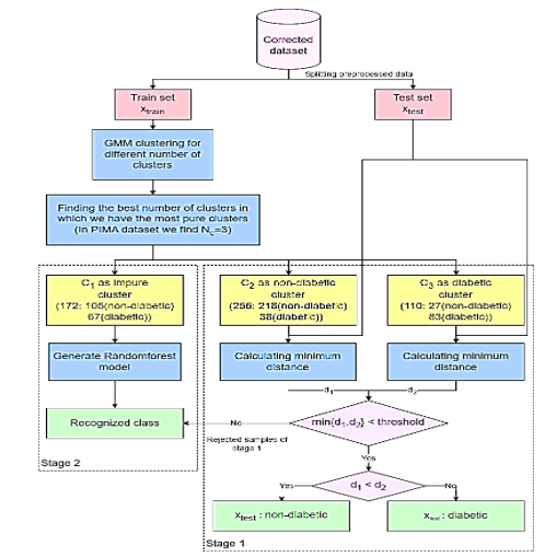 Figure 3. The flow diagram of the proposed semi-supervised classification method |
Results
Datasets
The PIMA Indian dataset utilized in this research comprises information from 768 instances of adult women aged 21 and older. This dataset includes various features, such as glucose level, blood pressure, skin thickness, insulin level, BMI, age, and diabetes status named" outcome" which indicates whether an individual has diabetes (1) or does not have diabetes (1 or 0).
Based on the available data, it can be observed that 65.1% of the patients in the dataset are categorized as non-diabetic, while 34.9% are identified as diabetic. Table 2 provides a description of the PIMA Indian dataset. A heat map illustrating the Pearson correlation coefficients for all diabetes-related characteristics is presented in Figure 4, demonstrating the relationships between the various variables in the dataset.
It is important to acknowledge that certain attributes, like" Pregnancy", may contain zero values, while others must not include zero values to maintain data validity. The frequency of zero values in the features is presented in Table 3. Based on the information in Table 3, it is evident that both insulin and glucose have a substantial number of missing values. Given the nature of the dataset and the specific characteristics of diabetes, it is essential to address these zero values appropriately during data preprocessing.
Evaluation
The performance of the classification algorithm was evaluated using various metrics, such as accuracy, precision, recall and F1-score. These metrics will be briefly explained in the following sections.
Accuracy: This is calculated by dividing the total number of correct predictions by the total number of predictions. It can be expressed as follows:
Precision (Positive Predictive Value (PPV)): This term refers to the proportion of true positive (TP) diagnoses of diabetic patients out of all samples that the model classified as diabetic, regardless of whether these classifications were correct (TP) or incorrect (False positives (FP)).
Recall (Sensitivity Rate): This term is defined as the proportion of correctly diagnosed diabetic patients (TP) out of all actual diabetic cases in the dataset, including both those correctly identified by the model (TP) and those that were missed (False negatives (FN)).
F1-Score: The F1-score is a metric that combines precision and recall, taking into account both false positives (FP) and FN.
Missing value imputation
In this paper, we introduced a new unsupervised imputation method based on clustering. The first step involved separating records without missing values (Reference data) from the datasets. These reference records were employed to impute missing values in the remaining records.
Initially, all reference data were clustered using the GMM algorithm. The clustering analysis was conducted with various numbers of clusters (k), and the results are presented in Table 4. One important measure for evaluating cluster quality is ensuring adequate separation, which minimizes variability between diabetic and non-diabetic patients within each cluster.
Upon examining different clusters, it was observed that a significant proportion of individuals without diabetes were grouped together in one cluster, while those with diabetes were distributed among different groups alongside non-diabetic individuals. Consequently, two clusters (k=2) were deemed most suitable for the proposed MVI method. Subsequently, these two scenarios were utilized to fill in the missing values in the dataset.
To evaluate the impact of the proposed method for imputing missing values on the accuracy of classification results, various classification techniques have been employed alongside different strategies for handling missing data.
A comparison was conducted using various algorithms, including SVM, RF, DT and our classification approach. Additionally, different data imputation techniques were employed, such as removing records with missing values, filling in missing values with the average, and utilizing the proposed method for imputing missing values. The results of this comparison are presented in Table 5.
The experimental findings revealed that the proposed MVI method for significantly improved the accuracy of these classification techniques.


The proposed classification method
The PIMA dataset comprises two groups: "Diabetics," referring to individuals diagnosed with diabetes, and "non-diabetics," referring to those without diabetes. The dataset exhibits an imbalanced class distribution, with approximately 65.1% of the records categorized as "non-diabetics" and 34.9% categorized as "diabetics."
To achieve an even distribution of classes in both the train and test sets, a balanced sampling method is employed. For this purpose, a random selection of 70% of the "non-diabetics" class records and 70% from the "diabetics" class is used to create the train dataset. This ensures that our training dataset preserves the original class distribution of the data. The remaining 30% of records, which include both "diabetic" and "non-diabetic" entries form the test set.
This stratified random sampling enables us to maintain the original class distribution in both the train and test sets, thereby facilitating effective training and evaluation of classification methods for both classes. The testing dataset offers an unbiased assessment of the classification model’s performance, considering class imbalances that are similar to those in the train set.
The model was implemented using Python 3.11 within the PyCharm 2022.3.3 development environment. A variety of Python libraries were employed to facilitate different aspects of the workflow, including openpyxl, Numpy, scikit-learn, Matplotlib, pandas, seaborn, and Python's built-in random module for stratified sampling. Each machine learning model was evaluated under various hyperparameter configurations. The random forest algorithm, with a maximum depth of 5 and 50 estimators, achieved the best performance during hyperparameter tuning. Furthermore, both cross-validation and stratified random sampling were employed, with each method being conducted five.
The adjustments to the proposed classification method are detailed below.
Clustering the train dataset: The train dataset is clustered using the GMM method with different numbers of clusters (k), ranging from 2 to 5. This analysis reveals that how the records are distributed among the clusters. Moreover, this examination shows the distribution of records across the clusters, and each clustering implementation with k clusters yields different distributions of " diabetic" and" non-diabetic" records within the clusters. This clustering analysis helps us understand the underlying patterns within the train dataset and how the" diabetics" and" non-diabetics" records are distributed among the clusters. The outcomes of clustering implementation with different numbers of clusters are presented in Table 6.
Choosing the optimal clusters: According to the clustering results, the train datasets are divided into three clusters (k=3), as illustrated in Table 6. The second cluster (C_2) contains more "non-diabetic" records and the third one (C_3) contains a greater number of "diabetic" records. These two clusters are utilized for classification purposes. The first cluster (C_1) consists of a mixture of "diabetic" and "non-diabetic" records. This heterogeneous cluster is excluded from this stage of the classification process, as it does not provide clear guidance for classifying the test records. A two-dimensional (2D) plot of the clusters is presented is Figure 5 based on Glucose and BMI for better visualization. These two variables were chosen due to their significant impact on the outcome, as indicated by the heatmap in Figure 4.
The total number of records in the two clusters-diabetics and non-diabetics-used as the basis for classification is 366.
Classification of test data based on two specified clusters: To classify the test data, the distances between each test data point and all data points within the "diabetic" and "non-diabetic" clusters are calculated. The label for the test data is assigned based on the nearest data point within these two clusters.
To further validate these assignments based on distances, a threshold is taken into account. If the test data point is closer to the "diabetic" cluster and the distance from the test data to this cluster is less than a specific threshold, labeled as "diabetics". Similarly, if it is nearer to the "non-diabetic" cluster and also meets the distance threshold, it is classified as "non-diabetic."
The experiments were conducted across a range of threshold values from 0.1 to 1, and the classification performance was assessed and presented in Table 7.
Choosing the optimal threshold: It is important to identify an optimal threshold that minimizes the rate of rejected data while maintaining high accuracy. Striking a balance between these factors is essential; therefore, we have selected a threshold value of 0.4 in order to achieve a lower rejection rate with minimal impact on accuracy.
Rejection rate of unclassifiable data: Test data points whose distance to the nearest "diabetic" or "non-diabetic" category exceeds the specified threshold are labeled as "rejected". The classifications of these instances become uncertain due to their proximity to the selected cluster data points.
The rejection rate of the algorithm is calculated as the proportion of data that could not be classified in the previous stage. These rates for different threshold values are computed and presented in Table 7.
Rejected data points classification: The evaluation of the algorithm can be conducted solely on labeled data without considering the rejected data points. To improve the efficiency of the proposed algorithm, a separate mechanism is also implemented to classify the rejected data.
According to the experimental results presented in Table 5, the random forest algorithm demonstrated superior classification performance compared to other machine learning algorithms. Consequently, this particular algorithm was selected for classifying rejected data points.
|
Table 4. Implementation of Gaussian mixture model clusters on records without missing values (Ranging from 2 to 5)
 Table 5. Evaluation of machine learning algorithm performance utilizing various missing value imputation techniques  RMV: Removing records containing Missing Values; FAV: Filling in missing values using the Average Value; PMVI: Proposed Missing Value Imputation method; SVM: Support Vector Machine; RF: Random Forest; DT: Decision Tree |
The unclassified data that has been excluded due to its greater distance from the diabetic and non-diabetic clusters is not sufficiently similar to be classified within these groups. Therefore, the most appropriate data for constructing a classification model for this excluded portion is the data from the first cluster (Table 6).
The first cluster data is utilized to train a random forest algorithm and create a classification model for the unclassified data points that were rejected, as they are more similar to this cluster than to the diabetic and non-diabetic clusters.
Evaluation of the proposed method: According to the details provided, each test data point is classified according to its proximity to the "diabetic" and "non-diabetic" clusters. If a data point is not classified at this stage, it receives a label from the model generated by the RF algorithm. After all test data have been labeled, the performance of the proposed algorithm is evaluated by calculating metrics such as accuracy, precision, recall, and F1-score. The entire proposed approach achieved an accuracy of 84%, as demonstrated in Table 8.
The proposed algorithm has been implemented five times for validation. Each iteration involves dividing the dataset into train and test, followed by applying all steps of the proposed algorithm. The results of each execution are presented in Table 8 and Figure 6.
The final accuracy, precision, recall, and F1-score for the algorithm are calculated as the average outcomes from five iterations of the algorithm.
|
Table 6. The implementation of Gaussian mixture model clusters on the train dataset (Ranging from 2 to 5)
 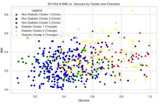 Figure 5. Visualization of optimal clusters (k=3) Table 7. The accuracy and the number of labeled and rejected records for proposed method using a range of threshold values from 0.1 to 1 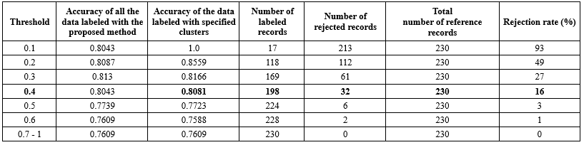 Re: Repetition; Avg: Average |
Comparing the proposed method to other methods
To gain a comprehensive understanding of the efficacy of our method in comparison to alternative approaches, we can refer to Tables 9 and 10, which provide a detailed analysis. These tables compare the proposed method, which employs the GMM and RF, with other classification techniques. To further evaluate the performance of the proposed method, an additional dataset was utilized alongside the PIMA dataset. The selected dataset, the Breast Cancer Wisconsin (Diagnostic) Dataset, comprises 569 patient records with 32 features. The target variable, diagnosis, indicates whether the cancer is benign (B) or malignant (M). The analysis results are summarized in Table 10.
To gain a comprehensive understanding of the efficacy of our method in comparison to alternative approaches, we can refer to Tables 9 and 10, which provide a detailed analysis. These tables compare the proposed method, which employs the GMM and RF, with other classification techniques. To further evaluate the performance of the proposed method, an additional dataset was utilized alongside the PIMA dataset. The selected dataset, the Breast Cancer Wisconsin (Diagnostic) Dataset, comprises 569 patient records with 32 features. The target variable, diagnosis, indicates whether the cancer is benign (B) or malignant (M). The analysis results are summarized in Table 10.
|
Table 8. Repeating the proposed method for five times
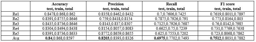 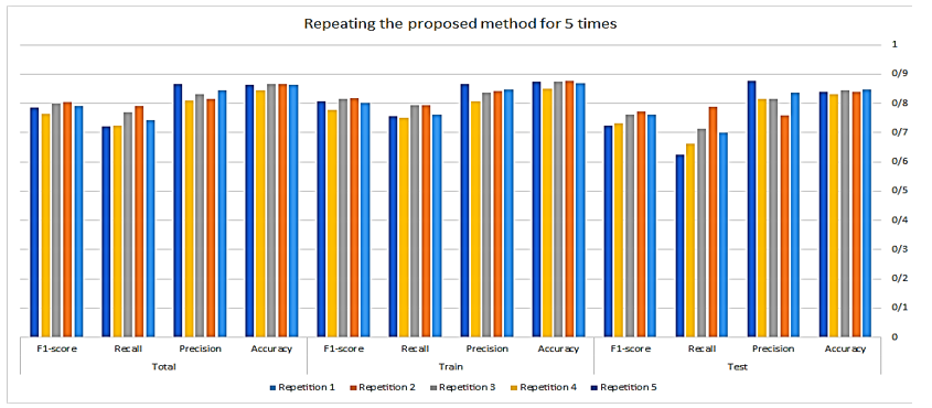 Figure 6. The comparison chart of the evaluation criteria of the proposed method for the total, train, and test datasets Table 9. Comparing the proposed method on the PIMA dataset to other methods  FS: Feature Selection, MVI: Missing Value Imputation, P: Precision, R: Recall, Fs: F1-score, Se: Sensitivity, Sp: Specificity, Acc: Accuracy; KNN: K-Nearest Neighbors; PCA: Principal Component Analysis; RB-Bayes: Recursive Bayesian; LR: Loistic Regression; RF: Random Forest; ANN: Artificial Neural Networks; NSGA: Non-dominated Sorting Genetic Algorithm; LDA: Linear Discriminant Analysis; GPC: Granite Powder Concrete; MLP: Multilayer Perceptron; EBBM-based UTM: Evolutionary Bait Balls Model-based unorganized Turing machine; KNN: K-Nearest Neighbor |
|
Table 10. Comparing the proposed method on the breast cancer dataset to other methods
 FS: Feature Selection; MVI: Missing Value Imputation; P: Precision’ R: Recall’ Fs: F1-score’ Se: Sensitivity; Sp: Specificity; Acc: Accuracy; SVM: Support Vector Machine; HCRF: Hierarchical Clustering Random Forest; LDA: Linear Discriminant Analysis; VIM: Variable Importance Measure; RF: Random Forest |
The efficiency of the proposed algorithm on the PIMA dataset is compared to state-of-the-art algorithms, as illustrated in Table 9. The results indicate that the proposed algorithm outperforms the state-of-the-art algorithms in terms of accuracy. Moreover, Table 10 shows that the proposed approach outperformed related techniques on the Wisconsin Diagnostic Breast Cancer (WDBC) dataset as well.
Discussion
The proposed approach accurately predicts categories of diabetic and non-diabetic individuals. This section provides an in-depth assessment of the influence of each component of the proposed method, highlighting their essential roles in achieving optimal outcomes.
The classifier is initially evaluated without applying a threshold in Stage 1 and without a classifier in Stage 2. Two datasets, each employing various MVI approaches, were created to evaluate predictions under varying conditions. The first dataset imputed missing values for a specific feature using the mean value of that feature from records belonging to the same class (Diabetic or non-diabetic) as the record with the missing value. In contrast, the second dataset utilized a proposed method for imputing missing values. The results presented in Table 11 demonstrate that the clustering-based approach significantly enhances predictions for both diabetic and non-diabetic classes, culminating in improved performance metrics.
|
Table 11. The impact of each component of the proposed approach on the results
 MVC: Missing Value Correction; UTS1C: Using Threshold in Stage 1 of Classification; CS2: Classifier in Stage 2; Acc: Accuracy; P: Precision; R: Recall; Fs: F1-score; Rel: Reliability; DT: Decision Tree; SVM: Support Vector Machines; RF: Random Forest |
A comparison was conducted between the prediction results with and without a threshold in Stage 1 of the proposed method for both datasets. As shown in Table 11, the implementation of a threshold improves the identification of records that are in close proximity, leading to enhanced performance. Conversely, without a threshold, there is a risk of misclassifying some records due to their dissimilarity.
Finally, in the second stage of the study, various classification methods were evaluated. The findings suggested that the RF algorithm would yield superior results. Consequently, data nodes with lower similarity to classifier clusters are flagged as rejected and their categories are forecasted using the RF algorithm, which demonstrated better performance compared to other machine learning techniques, as shown in Tables 5 and 11.
In summary, the proposed approach for addressing missing values, along with the suggested classification method, has improved diabetes prediction, yielding superior evaluation metrics compared to methods that do not incorporate these strategies. This underscores the significant benefits derived from their application.
Conclusion
In this study, we proposed a semi-supervised predictive model aimed at improving the accuracy of diabetes prediction using the PIMA dataset. Initially, we employed a clustering-based data imputation model to address missing values. The application of GMM to fill in these gaps was intended to enhance the integrity of the dataset, thereby providing a more reliable foundation for subsequent analytical processes.
Following the initial data preparation phase, a novel approach that combines clustering and classification methods has been proposed for predicting diabetes status. The classifier, which incorporates both GMM and RF algorithms, demonstrates improved predictive capability in identifying diabetes cases.
The consecutive implementation of these methods culminated in a significant accuracy rate of 86% in forecasting diabetes outcomes, positioning our developed model as a potential tool for categorizing diabetes cases.
One of the key challenges of the proposed approach is selecting optimal clusters, as the performance is highly sensitive to the chosen cluster configuration. Additionally, the computational cost of the method can pose difficulties when applied to large datasets. However, this limitation can be alleviated by employing optimizations, such as dimensionality reduction techniques.
Overall, the proposed algorithm demonstrates promising results, outperforming state-of-the-art algorithms in terms of accuracy for predicting diabetes. Furthermore, the method has proven effective when applied to other datasets, as evidenced by its success on an additional dataset tested during this study. Nonetheless, achieving the desired outcomes necessitates making well-informed and optimal decisions at each stage of the methodology.
Acknowledgement
The authors would like to thank all individuals who contributed indirectly to this research through their insights and discussions.
Funding sources
This research received no external funding.
Ethical statement
This study does not involve human participants or animal subjects requiring ethical approval. The data used in this research were obtained from publicly available sources.
Conflicts of interest
No conflict of interest.
Author contributions
FB conceived and designed the study, and HSh performed the data analysis and developed the models. Both authors contributed to the interpretation of the results, participated in writing the manuscript, and reviewed and approved the final version.
Data availability statement
The data is available at https://www.kaggle.com/datasets/uciml/pima-indians-diabetes-database.
Type of Article: Original article |
Subject:
Bio-statistics
Received: 2024/09/25 | Accepted: 2025/02/15 | Published: 2025/12/8
Received: 2024/09/25 | Accepted: 2025/02/15 | Published: 2025/12/8
References
1. Khan RMM, Chua ZJY, Tan JC, Yang Y, Liao Z, Zhao Y. From pre-diabetes to diabetes: Diagnosis, treatments and translational research. Medicina. 2019;55(9):546. [View at Publisher] [DOI] [PMID] [Google Scholar]
2. American Diabetes Association. Diagnosis and Classification of Diabetes Mellitus. Diabetes Care. 2010;33(Suppl_1):S62-9. [View at Publisher] [DOI] [PMID] [Google Scholar]
3. Marciano L, Camerini AL, Schulz PJ. The Role of Health Literacy in Diabetes Knowledge, Self-Care, and Glycemic Control. J Gen Intern Med. 2019;34(6):1007-1017. [View at Publisher] [DOI] [PMID] [Google Scholar]
4. Pantalone KM, Hobbs TM, Wells BJ, Kong SX, Kattan MW, Bouchard J, et al.Clinical characteristics, complications, comorbidities and treatment patterns among patients with type 2 diabetes mellitus in a large integrated health system. BMJ Open Diabetes Res Care. 2015;3(1):e000093. [View at Publisher] [DOI] [PMID] [Google Scholar]
5. World Health Organization. Diabetes. 2024 [View at Publisher]
6. International Diabetes Federation. Diabetes Atlas. 3rd ed. International Diabetes Federation;2007. [View at Publisher] [Google Scholar]
7. Franciosi M, Berardis GD, Rossi MCE, Sacco M, Belfiglio M, Pellegrini F, et al. Use of the diabetes risk score for opportunistic screening and impaired glucose tolerance. Diabetes Care. 2005;28(5):1187-94. [View at Publisher] [DOI] [PMID] [Google Scholar]
8. Huang Y, McCullagh P, Black N, Harper R. Feature selection and classification model construction on type 2 diabetic patient's data. Artif Intell Med. 2007;41(3):251-62. [View at Publisher] [DOI] [PMID] [Google Scholar]
9. Bellazzi R, Larizza C, Magni P, Montani S, Stefanelli M. Intelligent analysis of clinical time series: an application in the diabetes mellitus domain. Artif Intell Med. 2000;20(1):37-57. [View at Publisher] [DOI] [PMID] [Google Scholar]
10. Bellazzi R. Telemedicine and Diabetes Management: Current Challenges and Future Research Directions. J Diabetes Sci Technol. 2008;2(1):98-104. [View at Publisher] [DOI] [PMID] [Google Scholar]
11. Goel R, Misra A, Kondal D, Pandey RM, Vikram NK, Wasir JS, et al. Identification of insulin resistance in Asian Indian adolescents:classification and regression tree (CART) and logisticregression based classification rules. Clin Endocrinol (Oxf). 2009;70(5):717-24. [View at Publisher] [DOI] [PMID] [Google Scholar]
12. Heikes KE, Eddy DM, Arondekar B, Schlessinger L. Diabetes Risk Calculator,A simple tool for detecting undiagnosed diabetes and prediabetes. Diabetes Care. 2008;31(5):1040-5. [View at Publisher] [DOI] [PMID] [Google Scholar]
13. Rajni R, Amandeep A. RB-bayes algorithm for the prediction of diabetic in PIMA Indian dataset. International Journal of Electrical and Computer Engineering. 2019;9(6):4866-72. [View at Publisher] [DOI] [Google Scholar]
14. Lella L, Licata I, Pristipino C. Pima Indians Diabetes Database Processing through EBBM-Optimized UTM Model. In Proceedings of the 15th International Joint Conference on Biomedical Engineering Systems and Technologies- Volume 5: BIOSTEC, 384-9, 2022. [View at Publisher] [DOI] [Google Scholar]
15. Benarbia M. A Machine Learning Approach to Predicting the Onset of Type II Diabetes in a Sample of Pima Indian Women. The City University of New York. 2022. [Thesis, Master's capstone project] [View at Publisher] [Google Scholar]
16. Huang R. Prediction of Pima Indians Diabetes with Machine Learning Algorithms. University of California, Los Angeles. 2021. [Thesis] [View at Publisher] [Google Scholar]
17. Chang V, Bailey j, Ariel Xu Q, Sun Z. Pima Indians diabetes mellitus classification based on machine learning (ML) algorithms. Neural Comput Appl. 2022:1-17. [View at Publisher] [DOI] [PMID] [Google Scholar]
18. Alam TM, Atif Iqbal M, Ali Y, Abdul Wahab, Ijaz S, Imtiaz Baig T, et al. A model for early prediction of diabetes. Informatics in Medicine Unlocked. 2019;16:100204. [View at Publisher] [DOI] [Google Scholar]
19. Singh N, Singh P. Stacking-based multi-objective evolutionary ensemble framework for prediction of diabetes mellitus. Biocybernetics and Biomedical Engineering. 2020;40(1):1-22. [View at Publisher] [DOI] [Google Scholar]
20. Maniruzzaman Md, Kumar N,Menhazul Abedin Md, Shaykhul Islam Md, Suri HS, El-Baz AS, et al. Comparative approaches for classification of diabetes mellitus data: machine learning paradigm. Comput Methods Programs Biomed. 2017:152:23-34. [View at Publisher] [DOI] [PMID] [Google Scholar]
21. Kumari S, Kumar D, Mittal M. An ensemble approach for classification and prediction of diabetes mellitus using soft voting classifier, International Journal of Cognitive Computing in Engineering. 2021;2(1):40-6. [View at Publisher] [DOI] [Google Scholar]
22. Rajendra P, Latifi S. Prediction of diabetes using logistic regression and ensemble techniques. Comput Methods Programs Biomed Update. 2021;1:100032. [View at Publisher] [DOI] [Google Scholar]
23. Saxena R, Sharma SK, Gupta M, Sampada GC. A Novel Approach for Feature Selection and Classification of Diabetes Mellitus: Machine Learning Methods. Comput Intell Neurosci. 2022:2022:3820360. [View at Publisher] [DOI] [PMID] [Google Scholar]
24. Tigga NP, Garg S. Prediction of Type 2 Diabetes using Machine Learning Classification Methods. Procedia Computer Science. 2020;167:706-16. [View at Publisher] [DOI] [Google Scholar]
25. Chang V, Bailey j, Ariel Xu Q, Sun Z. Pima Indians diabetes mellitus classification based on machine learning (ML) algorithms. Neural Comput Appl. 2022:1-17. [View at Publisher] [DOI] [PMID] [Google Scholar]
26. Jackins V, Vimal S, Kaliappan M, Young Lee M. AI-based smart prediction of clinical disease using random forest classifer and Naive Bayes. J Supercomput. 2021;77:5198-5219. [View at Publisher] [DOI] [Google Scholar]
27. Patela E, Kushwaha DS. Clustering Cloud Workloads: K-Means vs Gaussian Mixture Model. Procedia Comput Sci. 2020;171:158-67. [View at Publisher] [DOI] [Google Scholar]
28. Fawagreh K, Medhat Gaber M, Elyan E. Random forests: from early developments to recent advancements. Syst Sci Control Eng. 2014;2(1):602-9. [View at Publisher] [DOI] [Google Scholar]
29. Olisah CC, Smith L, Smith M. Diabetes mellitus prediction and diagnosis from a data preprocessing and Machine Learning Perspective. Comput Methods Programs Biomed. 2022;220(9):106773. [View at Publisher] [DOI] [PMID] [Google Scholar]
30. Bhardwaj A, Bhardwaj H, Sakalle A, Uddin Z, Sakalle M, Ibrahim W. Tree-Based and Machine Learning Algorithm Analysis for Breast Cancer Classification. Comput Intell Neurosci. 2022:2022:6715406. [View at Publisher] [DOI] [PMID] [Google Scholar]
31. Adebiyi MO, Arowolo MO, Mshelia MD, Olugbara OO. A Linear Discriminant Analysis and Classification Model for Breast Cancer Diagnosis. Appl Sci. 2022;12(22):11455. [View at Publisher] [DOI] [Google Scholar]
32. Huang Z, Chen D. A Breast Cancer Diagnosis Method Based on VIM Feature Selection and Hierarchical Clustering Random Forest Algorithm. IEEE Access. 2021;10:3284-93. [View at Publisher] [DOI] [Google Scholar]
Send email to the article author
| Rights and permissions | |
 |
This work is licensed under a Creative Commons Attribution-NonCommercial 4.0 International License. |
